I've signed up for a half marathon and, as part of my training, have been looking for nearby slopes to run up. This post outlines how I used open data to find and compare the hilliest roads where I live.
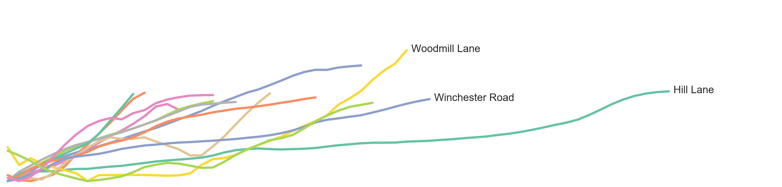
For example, here are elevation profiles of the roads in Edinburgh with biggest change in elevation (the difference between their highest and lowest points):
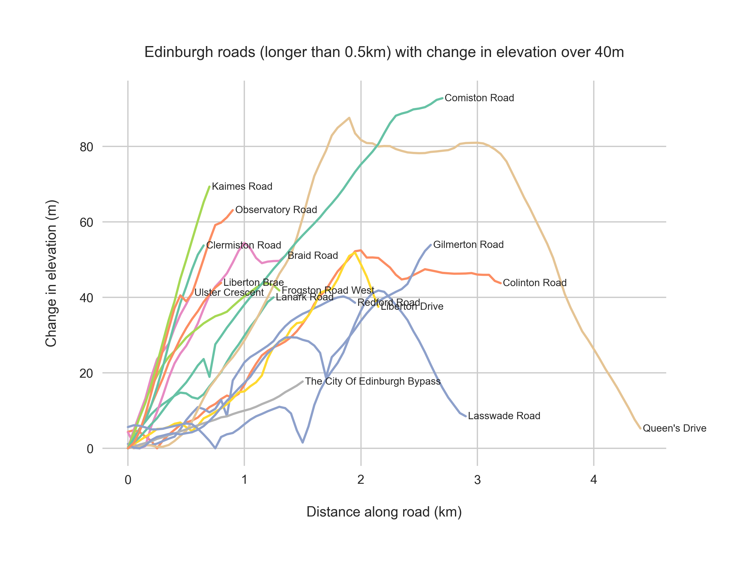
Queen's Drive loops around Arthur's Seat and Comiston Road skirts the Braid Hills.
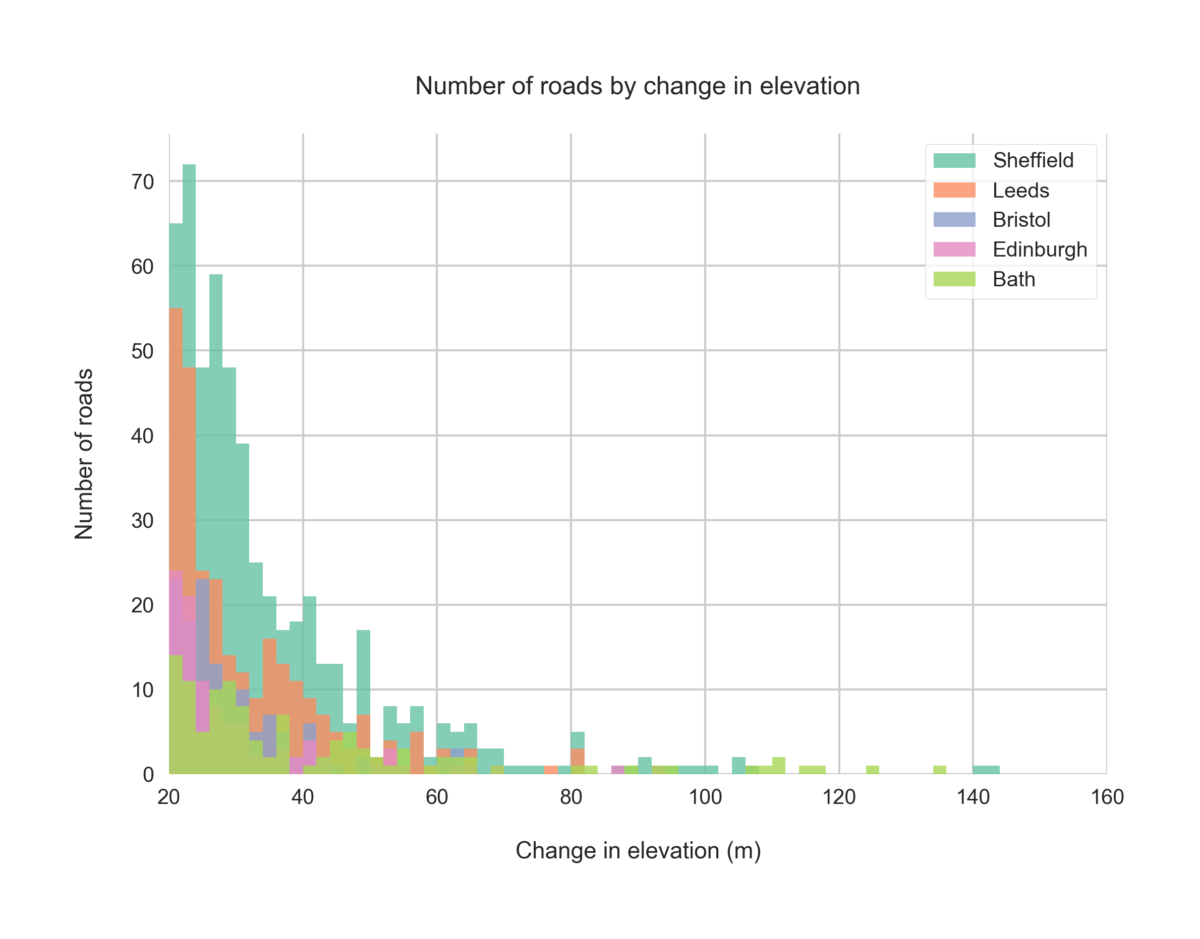
(Getting carried away / Avoiding doing any actual running,) I also compared a few UK cities to find the one wth hilliest roads. It's probably Sheffield, but Bath is up there too. This histogram shows five cities by the change in elevation of their roads:
Here's an overview of the process I used (the code is here).
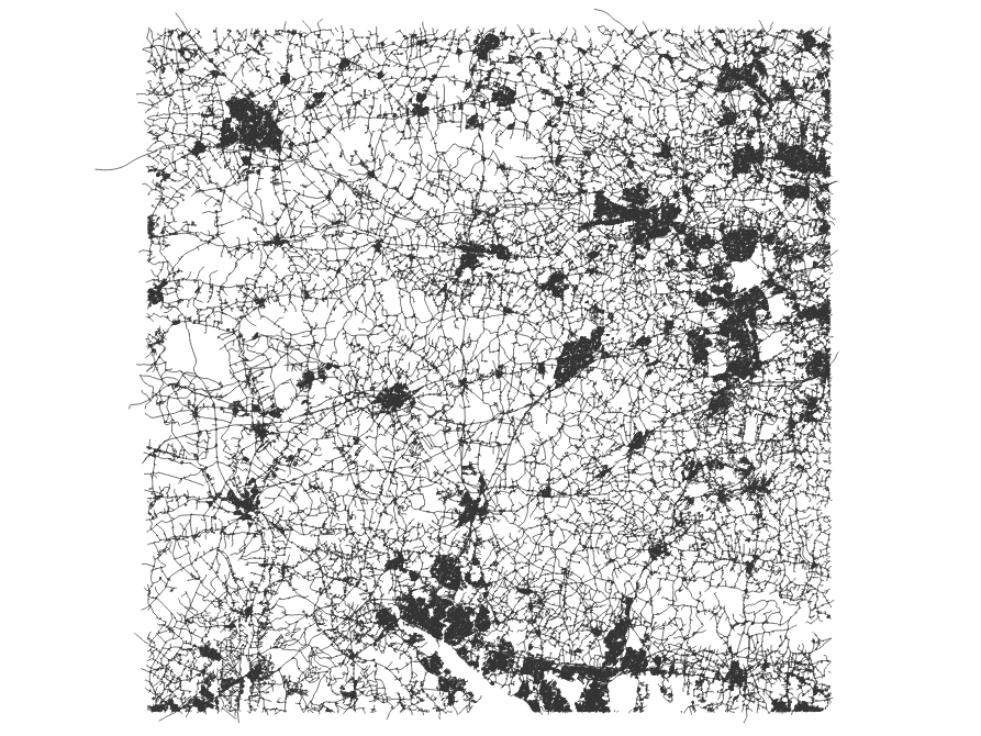
I started with Ordnance Survey's Open Roads, which is vector data on the UK's roads. Here's the SU square, covering Southampton (which I'll use as an example) in the south up to Didcot further north:
I also used OS's Boundary Line data to isolate only those roads within Southampton (GSS code: E06000045). This clipping is made easy with Geopandas (which uses Shapely for geometric operations and Fiona to read and write files):
roads = gpd.read_file("SU_RoadLink.shp")
boundary = gpd.read_file("district_borough_unitary_region.shp")
soton = boundary.loc[boundary["CODE"] == "E06000045"].reset_index()
soton_roads = roads[roads.geometry.within(soton.iloc[0].geometry)]
Here are the clipped roads:
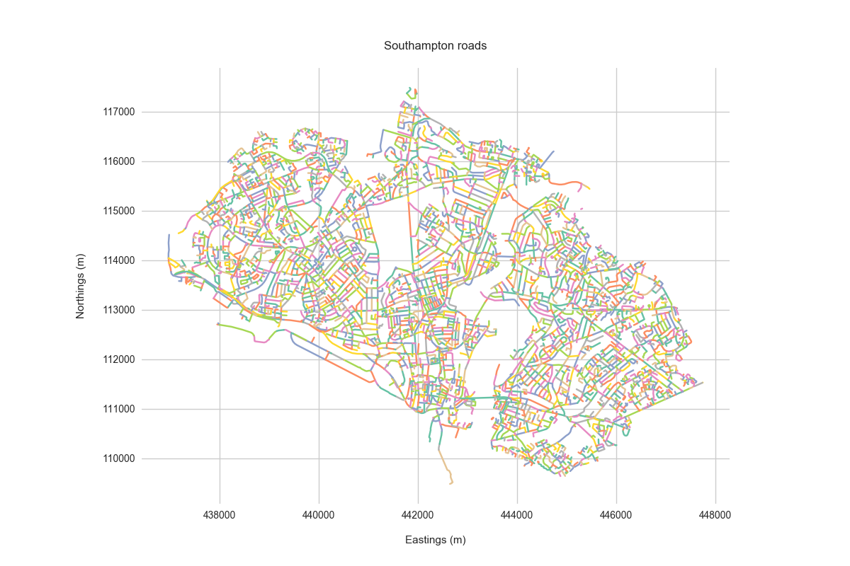
Open Roads represents the same road in many segments: a line for each stretch of road between junctions. I dissolved these segments into one line (though some are still represented as multiple lines - usually due to loops in the road):
soton_roads_geom = soton_roads.dissolve(by="nameTOID")
OS Open Roads contains the easting and northing of points along each road. To get the height, I needed to draw on the Environment Agency's LiDAR data (Composite 2m DTM). This data comes as an Esri ASCII grid file covering 1 square km.
I downloaded the files required to cover Southampton, and loaded them into one fairly large Pandas DataFrame (pickling this object makes a file about 450MB) with the eastings and northings as column names and row indices:
data_list = []
file_paths = glob.glob(os.path.join("elevation_data", "*.asc"))
for file in file_paths:
    ncols = int(linecache.getline(file, 1).split()[1])
    nrows = int(linecache.getline(file, 2).split()[1])
    xllcorner = int(linecache.getline(file, 3).split()[1])
    yllcorner = int(linecache.getline(file, 4).split()[1])
    cellsize = int(linecache.getline(file, 5).split()[1])
    eastings = list(range(xllcorner, xllcorner + (ncols*cellsize), cellsize))
    northings = list(reversed(range(yllcorner, yllcorner + (nrows*cellsize), cellsize))) # xllcorner is at the bottom of the file, so read from the top, but reverse the indices
    data = pd.read_csv(file, sep=" ", skiprows=6, names=eastings, na_values=-9999)
    data.index = northings
    data_list.append(data)

elevation = pd.concat([df.stack() for df in data_list], axis=0).unstack()
The DataFrame for Southampton looks like this (this is the top of the last few columns, which confusingly corresponds to the bottom right of the elevation data - eastings as the column names, northings as the row indexes, but in reverse order):
        449990  449992  449994  449996  449998
...        ...     ...     ...     ...     ...
105000  14.078  14.102  14.113  14.165  14.200
105002  14.055  14.075  14.113  14.170  14.182
105004  14.033  14.068  14.122  14.167  14.190
105006  14.023  14.055  14.113  14.158  14.208
105008  14.040  14.060  14.090  14.148  14.195
[7500 rows x 7500 columns]
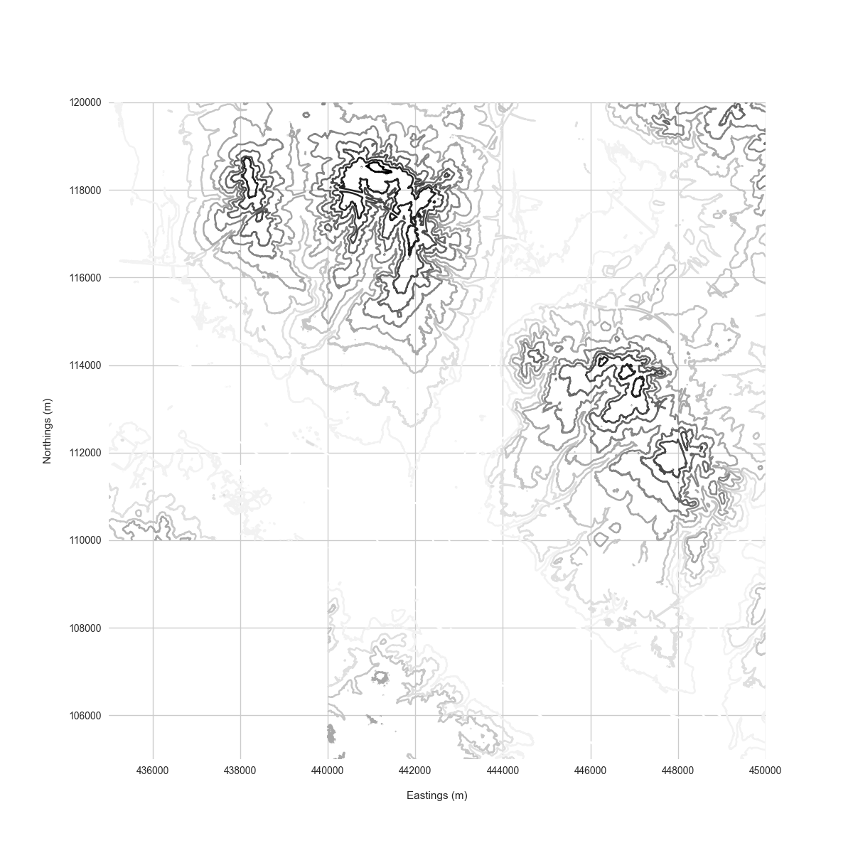
Here's the elevation data as a Matplotlib contour plot:
Once you have the roads and elevation datasets loaded, the next step is to loop through the roads and check the height at fixed intervals along each. Shapely's LineString.interpolate() makes this straightforward:
if line.length > 100: # Don't bother with tiny roads
    points = []
    for i in range(0, int(line.length), 50):
        ip = LineString(line).interpolate(i) # Interpolate along the road every 50m
        x, y = ip.xy
        x = round(x[0]/2)*2 # Round the easting and northing of the interpolated point to the nearest 2m
        y = round(y[0]/2)*2
        try:
            z = elevation.get_value(y, x) # Fetch the elevation at this point
        except KeyError:
            z = np.NaN
        points.append((x, y, z))
    new_line = LineString(points) # Make a new 3D LineString of the interpolated road
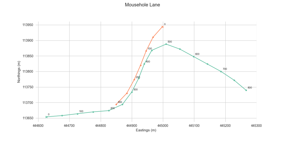
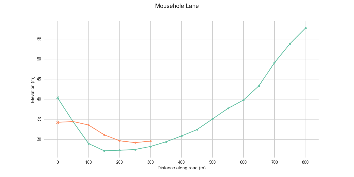
The new 3D lines are stored in the GeoPandas GeoDataFrame. Here's a plan view of Mousehole Lane, a fairly hilly road (with two non-continuous segments) in Southampton, with markers every 50m where the height was sampled:
Then the elevation profile of both segments:
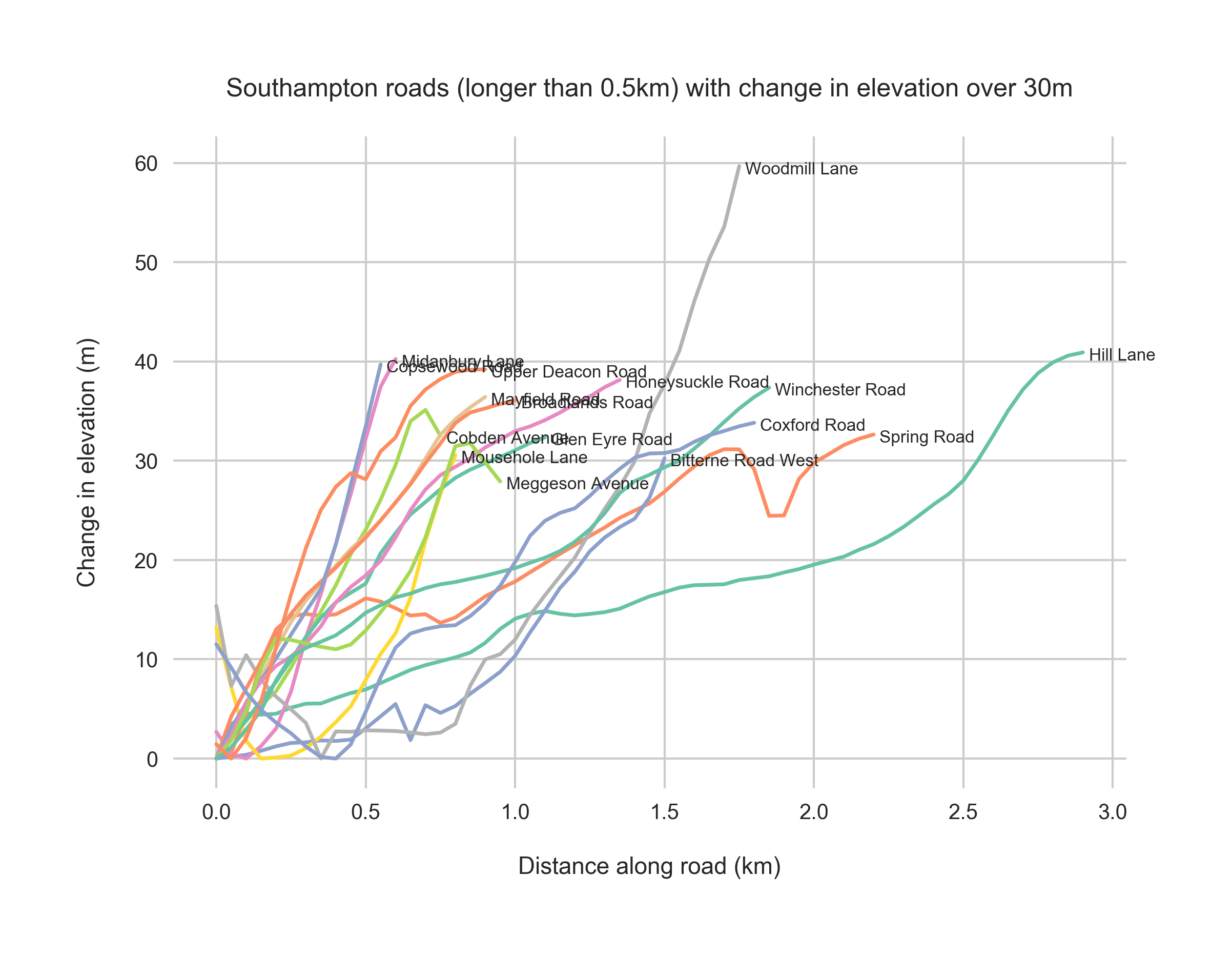
Southampton has sixteen roads with changes in elevation greater than 30m:
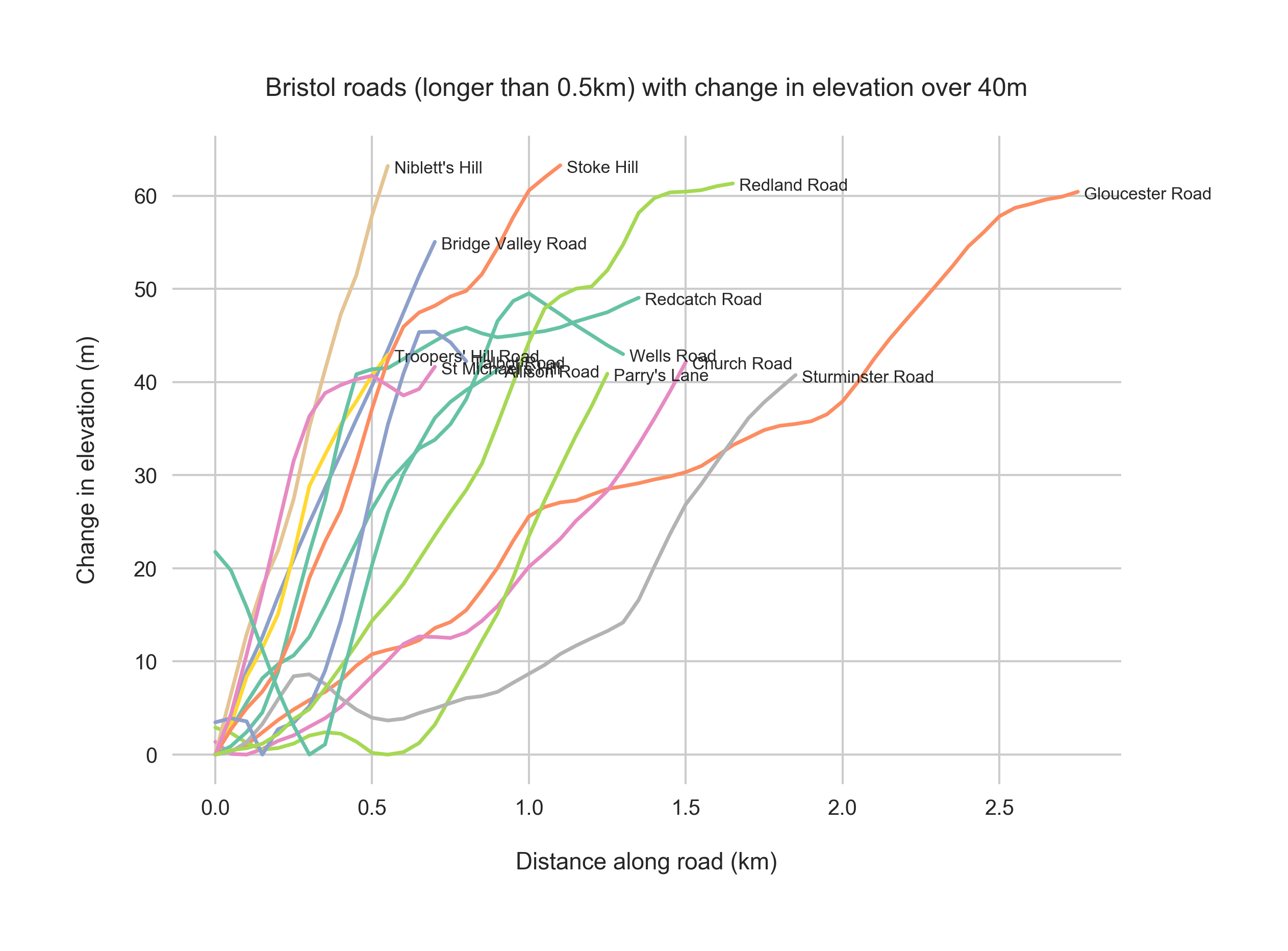
Bristol's fourteen hilliest roads:
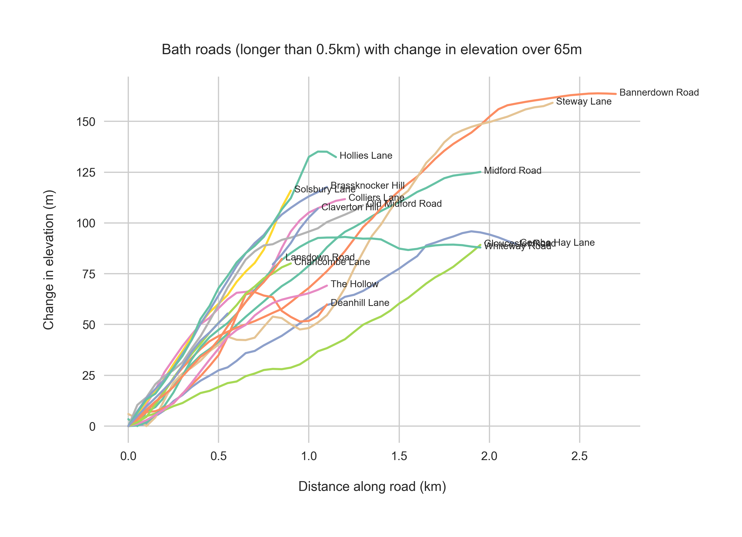
Bath's sixteen hilliest roads:
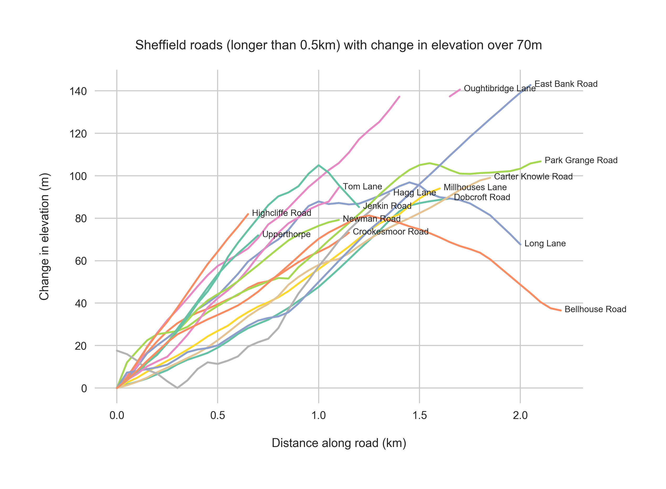
And Sheffield's fifteen hilliest roads:
Look here if you're interested in the full code.
The maps and charts on this page contain OS data © Crown copyright and database right 2017, as well as data which is © Environment Agency copyright and/or database right 2015. All rights reserved.